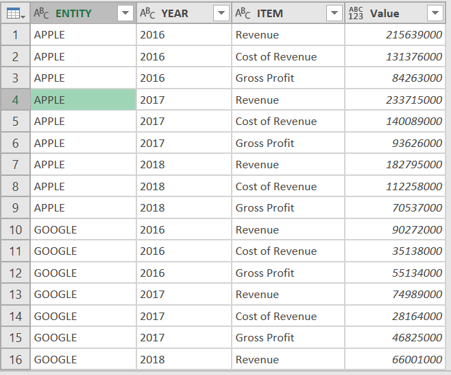
Following are the Revenue and Cost of Revenue of 3 Giant technology Companies for 3 years
| ENTITY | ITEMS | 2016 | 2017 | 2018 |
| APPLE | Revenue | 215,639,000 | 233,715,000 | 182,795,000 |
| APPLE | Cost of Revenue | 131,376,000 | 140,089,000 | 112,258,000 |
| Revenue | 90,272,000 | 74,989,000 | 66,001,000 | |
| Cost of Revenue | 35,138,000 | 28,164,000 | 25,691,000 | |
| MICROSOFT | Revenue | 85,320,000 | 93,580,000 | 86,833,000 |
| MICROSOFT | Cost of Revenue | 32,780,000 | 33,038,000 | 27,078,000 |
Your Objective is to Compute the Gross Profit (Revenue – Cost of Revenue) for each Company and Add it as a row to the Original Table. Following is the Final Output
| ENTITY | ITEM | 2016 | 2017 | 2018 |
| APPLE | Revenue | 215,639,000 | 233,715,000 | 182,795,000 |
| APPLE | Cost of Revenue | 131,376,000 | 140,089,000 | 112,258,000 |
| APPLE | Gross Profit | 84,263,000 | 93,626,000 | 70,537,000 |
| Revenue | 90,272,000 | 74,989,000 | 66,001,000 | |
| Cost of Revenue | 35,138,000 | 28,164,000 | 25,691,000 | |
| Gross Profit | 55,134,000 | 46,825,000 | 40,310,000 | |
| MICROSOFT | Revenue | 85,320,000 | 93,580,000 | 86,833,000 |
| MICROSOFT | Cost of Revenue | 32,780,000 | 33,038,000 | 27,078,000 |
| MICROSOFT | Gross Profit | 52,540,000 | 60,542,000 | 59,755,000 |
Power Query with its powerful Unpivot and Pivot features makes it very easy to do such stuff
Step#1: Load the Table in the Power Query
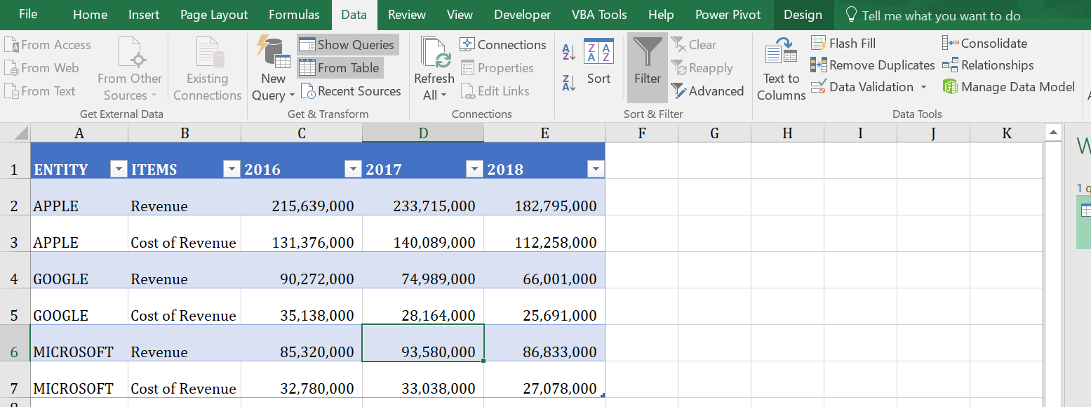
In Excel 2016…Go to Data Tab>>>Get & Transform>>> From Table
In previous versions of Excel you can use the “Power Query” tab
Picture Below shows this
Step2: Unpivot the Year Columns so that we have a single set of VALUES for pivoting in the next step
Select the year columns>>>Go to Transform tab >>>UNpivot
The picture below shows this
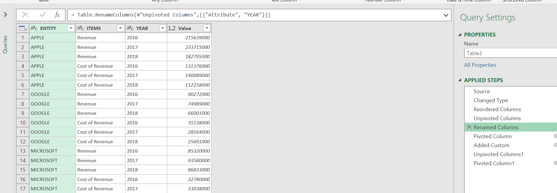
We get the YEARs unpivoted into a single Column. We rename this Column to YEARS. This is shown below
Step3: Pivot the Items Column so that we can compute the difference between Revenue and Cost of Revenue
Why? Because Power Query functions use Column references…..Unlike Excel there is no way to select a ROW or a cell
You might be thinking why do we not use Excel instead…..The answer is that …With Excel you can do it for sure…..but what if there were 500 countries. This will take you a substantial amount of time subtracting Cost of Revenue from Revenue for each and every entity. Power Query will do this in less than a minute
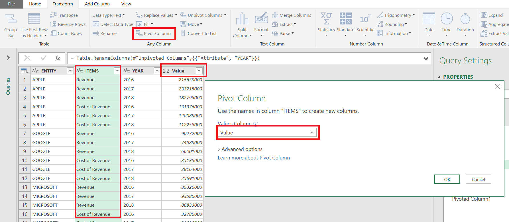
Select the ITEMS column>>> Go to Transform tab>>> PIVOT>>> Use Value Column as VALUES…………Picture below shows this
You will get the following
Step4: Now You can easily add a Column Gross Profit
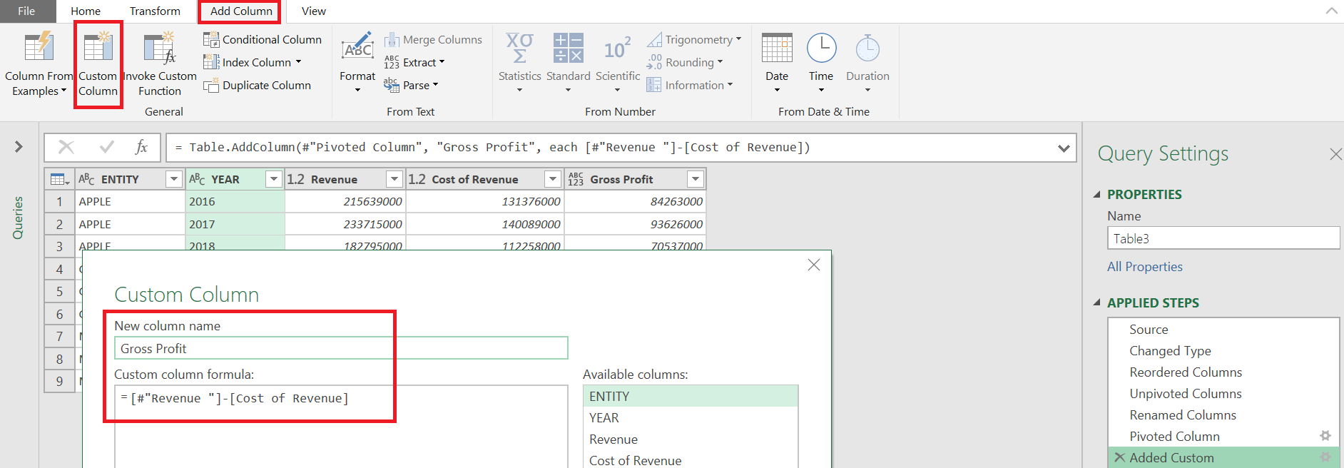
Go to “Add Column” tab>>> Custom Column……..Picture below shos this
Step5: Now you can Unpivot back the ITEM Columns
select the REVENUE/Cost of Revenue/Gross Profit Columns>>>>UNPIVOT
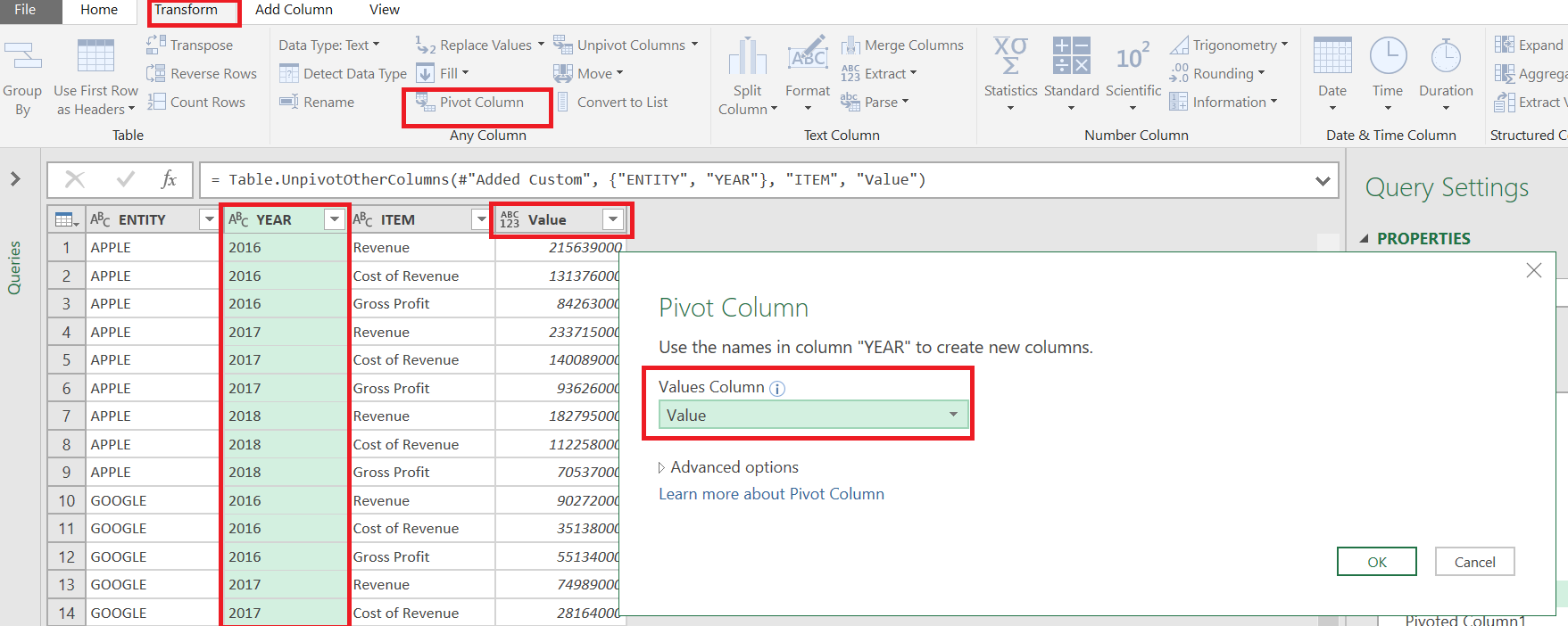
Step # 6: Final Step… You can Pivot back the YEARS column……..
Select the YEAR Column>>>Transform Tab>>> Pivot using VALUE column as VALUES
You will get the desired final output
Step#6 is not recommended though….. if you intend to use pivot tables with your final data Step #5 should be the final step
Click here to Download Excel file and see the steps in the Query Editor and play with them
