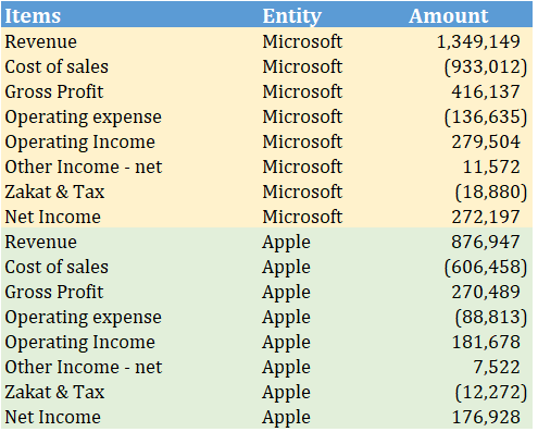
So we have this sample financial data of 2 technology giants..Microsoft and Apple
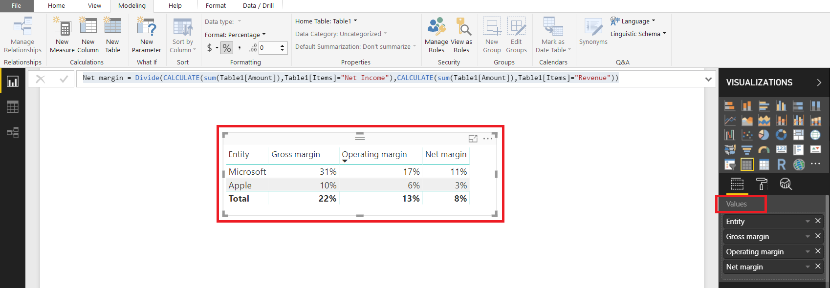
Using this Data we create 3 MEASURES to compute Profitability Ratios of these companies
Gross margin =
DIVIDE (
 CALCULATE ( SUM ( Table1[Amount] ), Table1[Items] = "Gross Profit" ),
 CALCULATE ( SUM ( Table1[Amount] ), Table1[Items] = "Revenue" )
)


Operating margin =
DIVIDE (
 CALCULATE ( SUM ( Table1[Amount] ), Table1[Items] = "Operating Income" ),
 CALCULATE ( SUM ( Table1[Amount] ), Table1[Items] = "Revenue" )
)


Net margin =
DIVIDE (
 CALCULATE ( SUM ( Table1[Amount] ), Table1[Items] = "Net Income" ),
 CALCULATE ( SUM ( Table1[Amount] ), Table1[Items] = "Revenue" )
)
You can put these MEASURES in “VALUES” section for any visual but
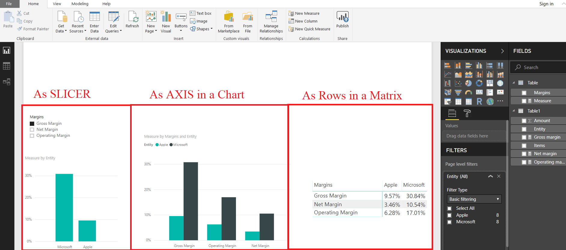
You can NOT put MEASURE in any other section like Slicers, Axis in a Chart or Rows of Matrix etc.
Only a column (including Calculated column) can be placed in Slicers, Axis in a Chart or Rows of Matrix etc.
But there is a trick to use MEASURES in slicers, Chart Axis or Matrix Rows etc
The trick is to create a separate table with a column containing the names of the MEASURES…and then create a formula to link MEASURES to these Column Values
FIRST STEP
Create a calculated table from the Modelling Tab to get MEASURE names in a column. (Alternatively you can manually create a Table by inputting information from Home Tab>>Enter Data)
Table =
DATATABLE (
 "Margins", STRING,
 {
 { "Gross Margin" },
 { "Operating Margin" },
 { "Net Margin" }
 }
)
STEP 2
Now we can create a MEASURE to link the Column Values to original profitability MEASURES
Measure =
VAR myvalue =
 SELECTEDVALUE ( 'Table'[Margins] )
RETURN
 SWITCH (
 TRUE (),
 myvalue = "Gross Margin", [Gross margin],
 myvalue = "Operating Margin", [Operating margin],
 myvalue = "Net Margin", [Net margin]
 )
STEP 3
Now you can use the combination of STEP 1 (Column created) and STEP 2 (MEASURE) to get the original MEASURES in SLICERS, Chart Axis, or Matrix Rows etc
DOWNLOAD
Click here to download the pbix File and play with it


