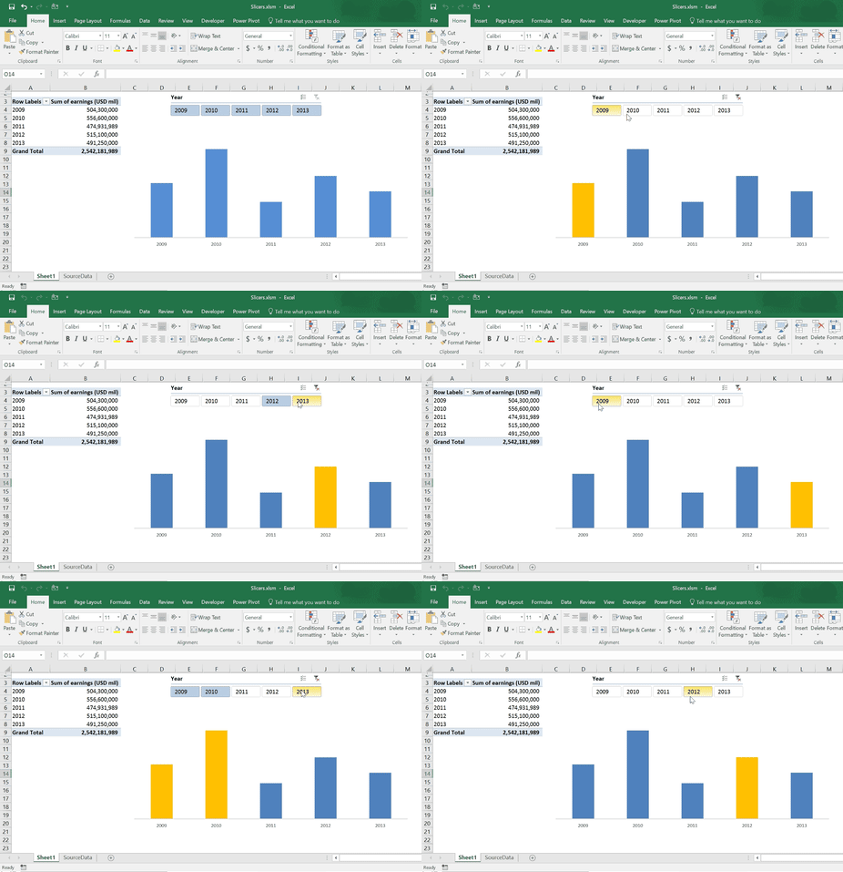
The normal behavior of slicer is to filter the associated Pivot Tables and Pivot Charts
How can we make Slicers HIGHLIGHT the selected items instead of applying them as FILTERS.
Power BI users know about this feature very well.Power BI allows you to “Edit Interactions” between visuals to either HIGHLIGHT or FILTER or DO NOTHING.
The animated image below shows what we are trying to achieve in Excel

This is DONE using “VBA” magic.
Here are the steps to do this
- Insert a slicer using the Pivot table on which chart is created
- Select and Copy this pivot table. Then paste a copy of it to separate location so that it is not visible in the DASHBOARD. Name this new Pivot table “DUMMY”
- Disconnect the SLICER from main PIVOT TABLE and Connect it to the DUMMY TABLE

4. I wrote the following code. What this code is that “It captures the position of the slicer item or items selected in an array. Then this array is used to highlight the related bars in the chart
Sub slicermacro()
On Error Resume Next
Dim Item As SlicerItem, myarray() As Integer, mychart As Chart, mysheet As Worksheet
Set mysheet = ActiveSheet
Set mychart = mysheet.ChartObjects(“Chart 2”).Chart
For i = 1 To ActiveWorkbook.SlicerCaches(“Slicer_Year1”).SlicerItems.Count
Set Item = ActiveWorkbook.SlicerCaches(“Slicer_Year1”).SlicerItems(i)
If Item.Selected = True Then
k = k + 1
ReDim Preserve myarray(1 To k)
myarray(k) = i
End If
Next i
mychart.SeriesCollection(1).ClearFormats
For i = 1 To UBound(myarray)
mychart.SeriesCollection(1).Points(myarray(i)).Format.Fill.ForeColor.RGB = RGB(255, 192, 0)
Next i
End Sub
5. Now we need to find an event when this macro would run. Unfortunately, no events are available for Slicers in Excel VBA. But events are available for Pivot Tables. Since now the slicer is connected to “DUMMY” pivot table we can use the Pivot Table Update event for “DUMMY” TABLE to run this macro
